You know what they say… Being great at Excel is actually just being great at Googling how to do things in Excel. We thought we would save you the trouble and put all the handy tricks in one spot to refer to. From basic tips like wrapping text and duplicating to data, to fancy tricks like creating drop down menus and graphs – we have got your Excel expertise sorted.

Everything we have compiled is simple to do but impressive to see. Let us transform your Excel experience into a breeze, and save you time and frustration. Here are our top ten tips and tricks to make you a spreadsheet whiz:

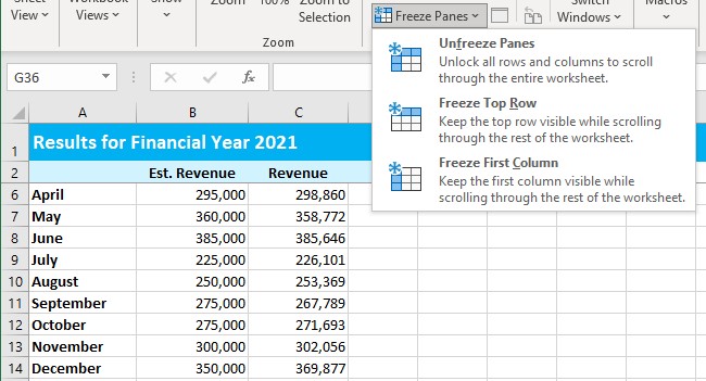
Freeze lines to remain visible while scrolling

Have you scrolled through rows of data only to forget which column is what without its header showing? You can freeze header rows to remain at the top of the spreadsheet as you scroll. Start by highlighting the row underneath the rows you want to keep visible, then jump up to the very top menu and select View. In the View toolbar, click Freeze Panes. This will freeze all the row above the row you highlighted.

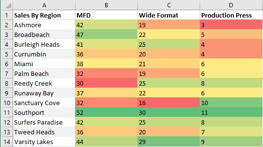
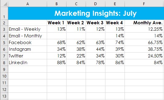
Conditional formatting

Visually format your data to reveal trends. Conditional formatting can display your data in an easy to interpret visual with colour scales, data bars, and icon sets. Simply highlight your data selection, jump up to your toolbar to click Conditional Formatting, then select how you want your data to be transformed. The above example uses Colour Scales, but you can also use Data Bars for a graph interpretation, or Icon Sets for green/red up/down arrows and more.

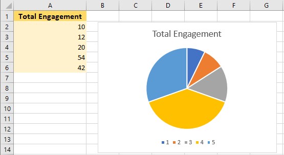
Create graphs in a flash

This one is lightning-fast. Select your column or row of data including the heading, then jump up the top to Insert, then select the type of graph you would like to create. Done!

You can also copy and paste these graphs straight into Microsoft Word. Just note, if you simply paste the graph into Word, it will update with any changes you make to the original graph in Excel. If you want to avoid these changes, use Paste Special and paste as a graphic.

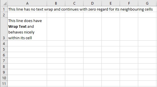
Text wrap within a cell

When you start typing in a cell, your text line defaults to having no text wrap and, as a result, continues the text line across the row over its neighbouring cells. If you want to keep your text confined to the outlines of its cell, select the cell, then in your toolbar at the top click Wrap Text. You can then select a text alignment just as you would in Microsoft Word. Once Wrap Text has been set, the text will remain within the cell and create line breaks where needed.

Same data across multiple cells

If you need the same data in multiple cells across your spreadsheet, you can! Start by selecting the cells you need either by a click and drag to select a portion of a column or row, or by selecting individual cells holding Ctrl. Once your cells are selected, type the data you need then hit Ctrl+Enter. Boom – all the selected cells will fill with the data you just input.

Duplicate the same data along a row or column

This is one everybody should know. If you want duplicate the exact same data across a row or down a column, simply type the value into the first cell, select the cell, then click the bottom right corner and drag to fill the newly highlighted cells. The data will be copied exactly as it is in the first cell you started at.

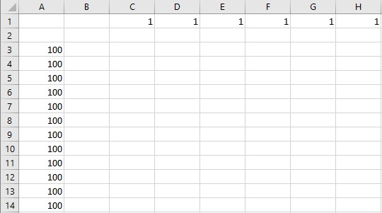
Start a data sequence along a row or column

The previous tip copied your value exactly, however, if you have a sequence of data to input such as months, dates, or simply increasing numbers, hold down Ctrl before you click and drag the bottom right corner.

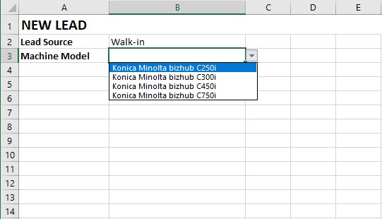
Create a drop down menu in a cell

We are getting a bit fancy now! If you have a spreadsheet you need others to fill out and you want to avoid all sorts of answers being input, a drop down menu is for you. Keep your data input by others totally consistent. Select the cell you want your drop down menu to live. At the very top menu, select Data. Navigate across to the Data Tools section and select Data Validation. A window will pop up: under Allow, select List. In the Source box, type your selections with a comma between each. Click OK. You now have a beautiful drop down menu to get the exact values you want!

Copy stylised cells with Format Painter

You’ve decide to add some style to your spreadsheet and completely changed the text, borders, and fill of a cell. To bring this same style across to other cells in your sheet, simply select the cell you jazzed up then click the paintbrush icon (Format Painter). Your style is now copied to the paintbrush and all you need to do is click the cell you want to transform.

If you want to transform more than one cell, instead of clicking a single cell, click and drag to make a selection of cells. This will transform all the cells you highlight to the style you created.

Best-ever shortcuts

This list of tricks would not be complete without a selection of shortcuts! Let’s cut to the chase:

Ctrl+; Insert the current date
Ctrl+Shift+# Change format of date
Ctrl+Shift+: Insert the current time
Ctrl+0 Hide the current column
Ctrl+9 Hide the current row
Ctrl+Shift+0 Unhide the current column (Highlight columns either side of hidden section first)
Ctrl+Shift+9 Unhide the current row (Highlight row either side of hidden section first)
F2 Start editing the selected cell (instead of double-clicking)
Ctrl+Spacebar Select entire column you are currently in
Shift+Spacebar Select entire row you are currently in
Ctrl+A Select entire spreadsheet
Ctrl+- Delete entire row or column selected, or entire spreadsheet if selected